Relatedness

NGSrelate - estimation of IBD probabilities

In order to estimate kinship coefficient then population allele frequencies are needed. These can be estimated from data if you can multiple individuals. For some individuals, for example most human populations, there are publicly available data. If you can obtain population allele frequencies or have a many samples from your population then we recommend that you use NGSrelate has works with ANGSD output. From the estimated IBD probabilities you can then infer the relationship. Below is a table of the expected IBD sharing probabilities assuming no inbreeding

Relationship	$K_{0}$	$K_{1}$	$K_{2}$
mono-zygotic twin	$0$	$0$	$1$
Parent-Offspring	$0$	$1$	$0$
Full siblings	$0.25$	$0.5$	$0.25$
Half siblings	$0.5$	$0.5$	$0$
First cousins	$0.75$	$0.25$	$0$
Unrelated	$1$	$0$	$0$

NGSrelate has its very own website http://www.popgen.dk/software/index.php/NgsRelate

IBS/genotype distribution

If you do not have population allele frequencies the you cannot estimate kinship coefficients. However, you can still make some claims about the relationship of your samples based on IBS patterns. Below is an example of IBS patterns between two individuals where we ignore the allele types. G is the genotype that counts for example the number of derived or non-reference alleles. Basically it is the 2D SFS where the is just 1 individual in each of the two populations

		ind2
ind1	$G=0$	$G=1$	$G=2$
$G=0$	$A$	$D$	$G$
$G=1$	$B$	$E$	$H$
$G=2$	$C$	$F$	$I$

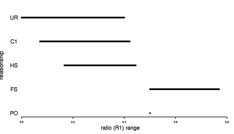
Here are some usefull ratio of IBS that can be used to say something about relatedness. Here we assume no inbreeding.

Relationship	Expected ratio	Expected ratio (R1)	Expected ratio (R1)
mono-zygotic twin	$B,C,D,F,G,H=0$	${\frac {E}{B+C+D+F+G+H}}=\infty$	-
Parent-Offspring	$C,G=0$	${\frac {E}{B+C+D+F+G+H}}=0.5$	-
Full siblings	${\frac {E}{C+G}}>10$	${\frac {E}{B+C+D+F+G+H}}>0.5$	${\frac {E}{B+C+D+F+G+H}}<10/13$
Half siblings	${\frac {E}{C+G}}>4$	${\frac {E}{B+C+D+F+G+H}}<4/9$	${\frac {E}{B+C+D+F+G+H}}>1/6$
First cousins	${\frac {E}{C+G}}>8/3$	${\frac {E}{B+C+D+F+G+H}}<8/19$	${\frac {E}{B+C+D+F+G+H}}>1/14$
Unrelated	${\frac {E}{C+G}}=2$	${\frac {E}{B+C+D+F+G+H}}<4/10$	${\frac {E}{B+C+D+F+G+H}}>0$

How to get the IBS pattern

You can get the estimate by using the 2D SFS method or you can use the genotype distribution method both in ANGSD.

The two methods are very similar but with a very small difference. The SFS method uses ancestral information or a reference in order to infer the 2 alleles for each position. The genotype distribution does not infer either the major or the minor allele but uses all 10 possible genotype likelihoods.

Rcode to get expectations

# R code go get expected IBS pattern
## k is the 3 IBD sharing probabities
## f is the allele frequency 
getEst<-function(k=c(1,0,0),f=0.5){
    p<-f
    q<-1-f
    m0<-rbind(
        c(p^4,2*p^3*q,p^2*q^2),
        c(2*p^3*q,4*p^2*q^2,2*p*q^3),
        c(p^2*q^2,2*q^3*p,q^4)
        )
   m1<-rbind(
        c(p^3,p^2*q,0),
        c(p^2*q,p^2*q+q^2*p,p*q^2),
        c(0,q^2*p,q^3)
        )
    m2<-rbind(
        c(p^2,0,0),
        c(0,2*p*q,0),
        c(0,0,q^2)
        )

return(k[1]*m0+k[2]*m1+k[3]*m2)

}

getEst(k=c(1,0,0),f=0.5)
       [,1]  [,2]   [,3]
[1,] 0.0625 0.125 0.0625
[2,] 0.1250 0.250 0.1250
[3,] 0.0625 0.125 0.0625