SFS Estimation

This method will estimate the site frequency spectrum, the method is described in Nielsen2012. The theory behind the model is briefly described here

This is a 2 step procedure first generate a ".saf" file (site allele frequency likelihood), followed by an optimization of the .saf file which will estimate the Site frequency spectrum (SFS).

For the optimization we have implemented 2 different approaches both found in the misc folder. The diagram below shows the how the method goes from raw bam files to the SFS.

NB the ancestral state needs to be supplied for the full SFS, but you can use the -fold 1 to estimate the folded SFS and then use the reference as ancestral.

The information on this page relates to versions 0.570 or higher.

In earlier version -doSaf was called -realSFS

<classdiagram type="dir:LR">

[sequence data{bg:orange}]->GL[genotype likelihoods|SAMtools;GATK;SOAPsnp;Kim et.al]

[genotype likelihoods|SAMtools;GATK;SOAPsnp;Kim et.al]->doSaf[.saf file{bg:blue}] [.saf file{bg:blue}]->optimize('emOptim2')[.saf.ml file{bg:red}]

</classdiagram>

Brief Overview

./angsd -doSaf 
	-> angsd version: 0.569	 build(Dec 17 2013 12:40:00)
	-> Analysis helpbox/synopsis information:
--------------
angsd_realSFS.cpp:
	-doSaf		0
	1: perform multisample GL estimation
	2: use an inbreeding version
	3: calculate genotype probabilities (beta)
	4: Assume genotype posteriors as input (still beta) 
	-doThetas		0 (calculate thetas)
	-underFlowProtect	0
	-fold			0 (deprecated)
	-anc			(null) (ancestral fasta)
	-noTrans		0 (remove transitions)
	-pest			(null) (prior SFS)

Options

-doSaf 1

Calculate the Site allele frequency likelihood based on individual genotype likelihoods assuming HWE

-doSaf 2

(version above 0.503) Calculate the Site allele frequency likelihood based on individual genotype likelihoods while taking into account individual inbreeding coefficients. This is implemented by Filipe G. Vieira

-doSaf 3

Calculate genotype probabilities

-doSaf 4

Assume genotype probs as intput (beta)

For the inbreeding version you need to supply a file containing all the inbreeding coefficients. -indF

-underFlowProtect [INT]

a very basic underflowprotection

Example

A full example is shown below, here we use GATK genotype likelihoods and hg19.fa as the ancestral. The emOptim2 can be found in the misc subfolder.

#first generate .saf file  with 4 threads
./angsd -bam bam.filelist -doSaf 1 -out small -anc  hg19.fa -GL 2 -P 4
#obtain a maximum likelihood estimate of the SFS using EM algorithm 
misc/emOptim2 small.saf 20 -maxIter 100 -P 4 >small.sfs

We always recommend that you filter out the bad qscore bases and meaningless mapQ reads. eg -minMapQ 1 -minQ 20.

If you have say 10 diploid samples, then you should choose 20
if you have say 12 diploid samples, then you should choose 24.

Interpretation of output file

The outpiles are then called small.em.ml. This will be the SFS in logscale. This is to be interpreted as:

column1 := probabilty of sampling zero derived alleles

column2 := probabilty of sampling one derived allele

column3 := probabilty of sampling two derived allele

column4 := probabilty of sampling three derived allele

etc

NB

The generation of the .saf file is done on a persite basis, whereas the optimization requires information for a region of the genome. The optimization will therefore use large amounts of memory. The program defaults to 50megabase regions, and will loop over the genome using 50 megebase chunks. You can increase this adding -nSites 500000000. Which will then use 500megabase regions.

Folded spectra

Below is for version 0.556 and above

If you don't have the ancestral state, you can instead estimate the folded SFS. This is done by supplying the -anc with the reference and also supply -fold 1. Then you should remember to change the second parameter to the emOptim2 function as the number of individuals instead of the number of chromosomes.

The above example would then be

#first generate .saf file
./angsd -bam bam.filelist -doSaf 1 -out small -anc  hg19.fa -GL 2 -fold 1 [options]
#now try the EM optimization with 4 threads
./emOptim2 small.saf 10 -maxIter 100 -P 4 >small.saf.em.ml

Posterior per-site distributions of the sample allele frequency

This is assuming version 0.556 or higher. If you supply a prior for the -doSaf analysis, the output of the .saf file will no longer be loglikeratios of the different categories but log posteriors of the different categories.

Format specification of binary .saf file

The information in this section is only usefull for people who wants to work with the "multisample GL"/"sample allele frequencies" for the individual sites.

Assuming 'n' individuals we have (2n+1) categories for each site, each value is encoded as ctype double which on 'all known' platforms occupies 8 bytes. The (2n+1) values are log scaled like ratios, which means that the most likely category will have a value of 0.

The information for the first site is the first (2n+1)sizeof(double) bytes. The information for the next site is the next (2n+1) bytes etc. The positions are given by the ascii file called '.saf.pos'

#sample code to read .saf in c/c++ assuming 10 individuals
FILE *fp = fopen("mySFS.saf","rb");
int nInd = 10;
double persite[2*nInd+1];
fread(persite,sizeof(double)*(2*nInd+1),1,fp);
for(int i=0;i<2*nind+1;i++)
   fprintf(stderr,"cat: %d = %f\n",i,persite[i]);

• If the -fold 1 has been set, then the dimension is no longer 2*nInd+1 but nInd+1
• If the -pest parameter has been supplied the output is no longer like ratios to the most likely but log posts of the different categories.

How to plot

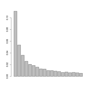
Assuming the we have obtained a single global sfs(only one line in the output) from emOptim2 program, and this is located in file.saf.sfs, then we can plot the results simply like:

sfs<-exp(scan("file.saf.sfs")) #read in the log sfs
barplot(sfs[-c(1,length(sfs))]) #plot variable sites 

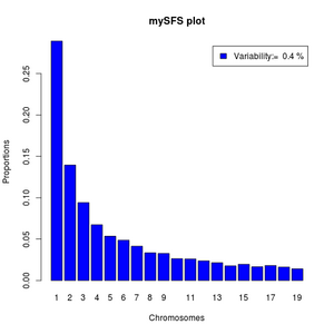
We can make it more fancy like below:

#function to normalize
norm <- function(x) x/sum(x)
#read data
sfs <- exp(scan("file.saf.sfs"))
#the variability as percentile
pvar<- (1-sfs[1]-sfs[length(sfs)])*100
#the variable categories of the sfs
sfs<-norm(sfs[-c(1,length(sfs))]) 
barplot(sfs,legend=paste("Variability:= ",round(pvar,3),"%"),xlab="Chromosomes",
names=1:length(sfs),ylab="Proportions",main="mySFS plot",col='blue')

If your output from emOptim2 contains more than one line, it is because you have estimated multiple local SFS's. Then you can't use the above commands directly but should first pick a specific row.

sfs<-exp(as.numeric(read.table("multiple.saf.sfs")[1,])) #first region.
#do the above
sfs<-exp(as.numeric(read.table("multiple.saf.sfs")[2,])) #second region.