ANGSD: Analysis of next generation Sequencing Data
Latest tar.gz version is (0.938/0.939 on github), see Change_log for changes, and download it here.
Error estimation: Difference between revisions
No edit summary |
|||
| (16 intermediate revisions by 2 users not shown) | |||
| Line 9: | Line 9: | ||
=Error estimation from polymorphic sites= | =Error estimation from polymorphic sites= | ||
The method for estimating | The method for estimating type specific errors is described in [[Kim2011]], and is based on the ''counts'' of the 4 different nucleotides. This method should be applied to the sites that are variable and the measure for variability is the simple MAF estimator that is described in [[Li2010]]. The idea of the method is briefly described [[errorSykMethod|here]] | ||
;NB | ;NB The analysis will use at least a prespecified number of sites (-minSites) for that analysis. If you do not have this number of variable sites, then the analysis will not be performed. | ||
The analysis will use at least | |||
==Brief Overview== | ==Brief Overview== | ||
| Line 33: | Line 32: | ||
==Options== | ==Options== | ||
; - | ; -minSites [int] | ||
default 10000. This is the number of sites we | default 10000. This is the minimum number of sites we used in the analysis. Every time this number of variable sites is read the error rates are estimated. This means that multiple error rates are estimated if the number of variable sites in you data exceeds the minimum number of sites. | ||
; - | ; -minPhat [float] | ||
default 0.005. This means we only run the error estimation on sites with a MAF>0.005. This should be modified according to the number of samples in the dataset. | default 0.005. This means we only run the error estimation on sites with a MAF>0.005. This should be modified according to the number of samples in the dataset. | ||
; -eps [float] | ; -eps [float] | ||
default 0.001.This is a guess of the | default 0.001.This is a guess of the error rate in the sample, this is used for the simple MAF estimator | ||
; -errors [filename] | ; -errors [filename] | ||
This file should contain a guess of the | This file should contain a start guess of the type specific errors. | ||
To further refine what data should be used please see [[alleles counts]]. | To further refine what data should be used please see [[alleles counts]] and [[input#Bam_files]]. | ||
==Example== | ==Example== | ||
The simplest example is: | The simplest example is: | ||
<pre> | <pre> | ||
./angsd -bam bam.filelist -doCounts 1 -out test -doError 1 -doMajorMinor 2 -nThreads | ./angsd -bam bam.filelist -doCounts 1 -out test -doError 1 -doMajorMinor 2 -nThreads 5 -minSites 1000 -r 1: | ||
</pre> | </pre> | ||
Or a more elaborate example where we only want to estimate the typespecific errors for the "good" data: | Or a more elaborate example where we only want to estimate the typespecific errors for the "good" data: | ||
<pre> | <pre> | ||
./angsd -bam bam.filelist -doCounts 1 -out test2 -doError 1 -doMajorMinor 2 -nThreads | ./angsd -bam bam.filelist -doCounts 1 -out test2 -doError 1 -doMajorMinor 2 -nThreads 5 -minSites 1000 -minQ 20 -minMapQ 30 -r 1: | ||
</pre> | </pre> | ||
| Line 72: | Line 71: | ||
0.001451 0.004327 0.000974 0.000000 | 0.001451 0.004327 0.000974 0.000000 | ||
</pre> | </pre> | ||
Notice that we for the more stringent test2 dataset have somewhat lower error rates. But we should really choose a much larger number of sites to do this analysis. Each line has 16 entries corresponding to the type specific errors for a region of '''- | Notice that we for the more stringent test2 dataset have somewhat lower error rates. But we should really choose a much larger number of sites to do this analysis. Each line has 16 entries corresponding to the type specific errors for a region of '''-minSites'''. | ||
NB Currently the ordering of each line, can not be interpreted as the error rates along the genome, due to the threading. This will likely change in future versions. | NB Currently the ordering of each line, can not be interpreted as the error rates along the genome, due to the threading. If no threading is used the order is preserved. This will likely change in future versions. | ||
We can visualise this easily in R, see figures on right side (These are not the values from the above) | We can visualise this easily in R, see figures on right side (These are not the values from the above) | ||
| Line 90: | Line 89: | ||
[[File:errorEstOverall.png|thumb]] | [[File:errorEstOverall.png|thumb]] | ||
The estimated rates can roughly be interpreted as relative error rates. That is excess of derived alleles in your sample compare to the derived alleles in the an error free indviduals The idea is the your sample and the error free individuals should have the same expected number of derived alleles and the extra observed derived alleles in you sample are due to the excess error. For each individual we sample a single base from the reads at each position. We use only positions were there are coverage for both the outgroup, the sample and the error free individual. | The estimated rates can roughly be interpreted as relative error rates. That is excess of derived alleles in your sample compare to the derived alleles in the an error free indviduals The idea is the your sample and the error free individuals should have the same expected number of derived alleles and the extra observed derived alleles in you sample are due to the excess error. For each individual we sample a single base from the reads at each position. We use only positions were there are coverage for both the outgroup, the sample and the error free individual. Some more details about the method is described [[ErrorPerfect|here]]. | ||
If you work with human data mapped to hg19 we have a fasta file containing the ancestral states (actually the chimp mapped to hg19). | |||
<pre> | |||
wget http://popgen.dk/software/download/angsd/hg19ancNoChr.fa.gz | |||
</pre> | |||
==Brief Overview== | ==Brief Overview== | ||
<pre> | <pre> | ||
./angsd -doAncError | ./angsd -doAncError | ||
-> angsd version: 0. | Command: | ||
./angsd -doAncError | |||
-> angsd version: 0.580 build(Feb 26 2014 10:11:49) | |||
-> Analysis helpbox/synopsis information: | -> Analysis helpbox/synopsis information: | ||
-------------- | -------------- | ||
analysisAncError.cpp: | analysisAncError.cpp: | ||
-doAncError 0 | -doAncError 0 | ||
(Sampling strategies) | |||
0: no error estimation | |||
1: (Use all bases) | |||
0: (Use all bases) | 2: (Sample single base) | ||
3: (Sample first base) | |||
Required: | Required: | ||
-ref (null) (fastafile containg 'perfect' sample) | -ref (null) (fastafile containg 'perfect' sample) | ||
-anc (null) (fastafile containg outgroup) | -anc (null) (fastafile containg outgroup) | ||
NB: the -ref should be a fasta for a sample where you assume no errors. | |||
We measure the difference between the outgroup and your -ref sample. | |||
The statistic is then the excess of substitutions between your BAM file and outgroup, compared to the perfect sample. After the ANGSD run use: Rscript R/estError.R file=angsdput.ancerror | |||
</pre> | </pre> | ||
| Line 113: | Line 122: | ||
==Options== | ==Options== | ||
; -doAncError | ; -doAncError [int] | ||
Use -doAncError to use this analysis | Use -doAncError to use this analysis. | ||
0: No error estimation | |||
1: Use all reads | |||
2: Sample only one base per site | |||
3: Use first read per site (the reads are order with position start) | |||
To further refine what data should be used please see [[alleles counts]] and [[Input | read filters]]. | |||
; -anc [filename] | ; -anc [filename] | ||
fasta file with the ancestral alleles | fasta file with the ancestral alleles | ||
; -ref [filename] | ; -ref [filename] | ||
fasta file of an error free individual. | fasta file of an error free individual. | ||
] | |||
==Example== | ==Example== | ||
| Line 138: | Line 151: | ||
<pre> | <pre> | ||
Rscript | Rscript R/estError.R file=output/smallBamMicsAncq30Q20.ancError main="Errorrate using outgroup (CHIMP) and a perfect MAN" doPng=TRUE | ||
</pre> | </pre> | ||
;NB the script will generate an empty Rplots.pdf file. This is expected. Sorry about this. The reason is that we haven't figured out how to change the R command called palette without generating a Rplots.pdf file. | ;NB the script will generate an empty Rplots.pdf file. This is expected. Sorry about this. The reason is that we haven't figured out how to change the R command called palette without generating a Rplots.pdf file (stupid R 3.+ color palette). | ||
==Output== | ==Output== | ||
# The output from the angsd cprogram is in a horrible format. Those are 2 files suffixed with '''*.ancError''' and '''*.ancErrorChr'''. | # The output from the angsd cprogram is in a horrible format. Those are 2 files suffixed with '''*.ancError''' and '''*.ancErrorChr'''. | ||
For each individual we allocate a integer vector with 125 entries. Each entry represents the counts of combinations of the outgroup,perfect,sample alleles. The offset is given by: outgroup*25+perfect*5+bam;With the bases encoded as a=0,c=1,g=2,t=3,n=4 | |||
# The Rscript will output the type specific errors and the overall errors. It will also produce two figures. One will the type specific errors and one with the overall errors. If a lot of individuals are included in the analysis the figure will need to be modified. The output is 3 files: 2) figures called '''errorEst/errorEstOverall'''. And a text file containing the values used for generating the figures. Example below | # The Rscript will output the type specific errors and the overall errors. It will also produce two figures. One will the type specific errors and one with the overall errors. If a lot of individuals are included in the analysis the figure will need to be modified. The output is 3 files: 2) figures called '''errorEst/errorEstOverall'''. And a text file containing the values used for generating the figures. Example below | ||
| Line 161: | Line 176: | ||
</pre> | </pre> | ||
= | =Mismatch rates= | ||
Type, strand, read position specific mismatch rates can be obtain using the [[Genotype_likelihoods#SOAPsnp | soapSNP genotype likelihood method]]. Use a reference genome with known variations removed to reduce the bias of this method | |||
Latest revision as of 12:57, 12 January 2017
ANGSD currently has 2 different methods for estimating error rates.
- A method that will estimate the joint typespecific errorrates for multiple samples. This method is using the minor allele frequency as prior, and therefore this method can not be used for single samples.
- A method that that uses an outgroup and an 'errorfree' individual. Useful for single samples.
The type specific errorrates is an matrix, with the error rates of observing base e.g. A when in reality the true base is e.g. C.
Error estimation from polymorphic sites
The method for estimating type specific errors is described in Kim2011, and is based on the counts of the 4 different nucleotides. This method should be applied to the sites that are variable and the measure for variability is the simple MAF estimator that is described in Li2010. The idea of the method is briefly described here
- NB The analysis will use at least a prespecified number of sites (-minSites) for that analysis. If you do not have this number of variable sites, then the analysis will not be performed.
Brief Overview
./angsd -doError
        -> angsd version: 0.564  build(Dec  6 2013 12:52:55)
        -> Analysis helpbox/synopsis information:
---------------------
analysisEstError.cpp:
-doError        0
        1: SYK method, joint typespecific errors (Multisample)
        -minSites       10000
        -errors         (null)  (Filename for starterrors)
        -emIter         100
        -minPhat        0.005000        (Minimum phat)
        -eps            0.001000        (Estimate of errorrate)
        NB this method requires -doMajorMinor 2
Options
- -minSites [int]
default 10000. This is the minimum number of sites we used in the analysis. Every time this number of variable sites is read the error rates are estimated. This means that multiple error rates are estimated if the number of variable sites in you data exceeds the minimum number of sites.
- -minPhat [float]
default 0.005. This means we only run the error estimation on sites with a MAF>0.005. This should be modified according to the number of samples in the dataset.
- -eps [float]
default 0.001.This is a guess of the error rate in the sample, this is used for the simple MAF estimator
- -errors [filename]
This file should contain a start guess of the type specific errors.
To further refine what data should be used please see alleles counts and input#Bam_files.
Example
The simplest example is:
./angsd -bam bam.filelist -doCounts 1 -out test -doError 1 -doMajorMinor 2 -nThreads 5 -minSites 1000 -r 1:
Or a more elaborate example where we only want to estimate the typespecific errors for the "good" data:
./angsd -bam bam.filelist -doCounts 1 -out test2 -doError 1 -doMajorMinor 2 -nThreads 5 -minSites 1000 -minQ 20 -minMapQ 30 -r 1:
Output
The output for this analysis is a file suffixed with *.error.chunkunordered.


#test
0.000000	0.005488	0.003847	0.003137\
0.006807	0.000000	0.001972	0.002396\
0.002190	0.001855	0.000000	0.008068\
0.002491	0.004268	0.005812	0.000000
#test2
0.000000	0.000071	0.003381	0.001254\
0.003989	0.000000	0.000000	0.002568\
0.002270	0.000000	0.000000	0.003650\
0.001451	0.004327	0.000974	0.000000
Notice that we for the more stringent test2 dataset have somewhat lower error rates. But we should really choose a much larger number of sites to do this analysis. Each line has 16 entries corresponding to the type specific errors for a region of -minSites.
NB Currently the ordering of each line, can not be interpreted as the error rates along the genome, due to the threading. If no threading is used the order is preserved. This will likely change in future versions.
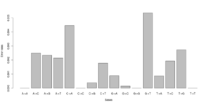
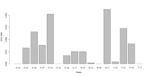
We can visualise this easily in R, see figures on right side (These are not the values from the above)
a <- as.numeric(read.table("test.error.chunkunordered",nrow=1))
b <- as.numeric(read.table("test2.error.chunkunordered",nrow=1))
DNA<-c("A","C","G","T")
names(a) <- as.vector((sapply(1:4,function(x) paste(DNA[x],DNA,sep="->"))))
barplot(a)
barplot(b)
Error estimation using an outgroup and an error free individual


The estimated rates can roughly be interpreted as relative error rates. That is excess of derived alleles in your sample compare to the derived alleles in the an error free indviduals The idea is the your sample and the error free individuals should have the same expected number of derived alleles and the extra observed derived alleles in you sample are due to the excess error. For each individual we sample a single base from the reads at each position. We use only positions were there are coverage for both the outgroup, the sample and the error free individual. Some more details about the method is described here.
If you work with human data mapped to hg19 we have a fasta file containing the ancestral states (actually the chimp mapped to hg19).
wget http://popgen.dk/software/download/angsd/hg19ancNoChr.fa.gz
Brief Overview
./angsd -doAncError
Command:
./angsd -doAncError
	-> angsd version: 0.580	 build(Feb 26 2014 10:11:49)
	-> Analysis helpbox/synopsis information:
--------------
analysisAncError.cpp:
	-doAncError	0
	(Sampling strategies)
	 0:	 no error estimation
	 1:	 (Use all bases)
	 2:	 (Sample single base)
	 3:	 (Sample first base)
Required:
	-ref	(null)	(fastafile containg 'perfect' sample)
	-anc	(null)	(fastafile containg outgroup)

NB: the -ref should be a fasta for a sample where you assume no errors.
We measure the difference between the outgroup and your -ref sample.
The statistic is then the excess of substitutions between your BAM file and outgroup, compared to the perfect sample. After the ANGSD run use:  Rscript R/estError.R file=angsdput.ancerror
To make matters explicit: For this analysis, the -ref should not be your reference, but a fasta file containing the consensus of a 'perfect' sample. The method will calculate the difference between the -ref and -anc, and the difference between the supplied BAM files, and interpret the excess of difference as an error. You can generate a consensus fasta with -doFasta.
Options
- -doAncError [int]
Use -doAncError to use this analysis. 0: No error estimation
1: Use all reads
2: Sample only one base per site
3: Use first read per site (the reads are order with position start)
To further refine what data should be used please see alleles counts and read filters.
- -anc [filename]
fasta file with the ancestral alleles
- -ref [filename]
fasta file of an error free individual. ]
Example
- angsd -doAncError 1 -anc chimpHg19.fa -ref hg19perfect.fa -out results -bam bam.filelist
- Rscript R/estError.R file=results.ancError
Typing Rscript R/estError.R will give you additional options for plotting the results.
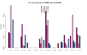
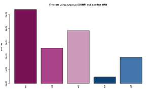
The command for plotting the figure on the right was given as:
Rscript R/estError.R file=output/smallBamMicsAncq30Q20.ancError main="Errorrate using outgroup (CHIMP) and a perfect MAN" doPng=TRUE
- NB the script will generate an empty Rplots.pdf file. This is expected. Sorry about this. The reason is that we haven't figured out how to change the R command called palette without generating a Rplots.pdf file (stupid R 3.+ color palette).
Output
- The output from the angsd cprogram is in a horrible format. Those are 2 files suffixed with *.ancError and *.ancErrorChr.
For each individual we allocate a integer vector with 125 entries. Each entry represents the counts of combinations of the outgroup,perfect,sample alleles. The offset is given by: outgroup*25+perfect*5+bam;With the bases encoded as a=0,c=1,g=2,t=3,n=4
- The Rscript will output the type specific errors and the overall errors. It will also produce two figures. One will the type specific errors and one with the overall errors. If a lot of individuals are included in the analysis the figure will need to be modified. The output is 3 files: 2) figures called errorEst/errorEstOverall. And a text file containing the values used for generating the figures. Example below
"C -> A"	"G -> A"	"T -> A"	"A -> C"	"G -> C"	"T -> C"	"A -> G"	"C -> G"	"T -> G"	"A -> T"	"C -> T"	"G -> T"
"ind1"	0.000288466623749173	1e-10	0.000205229813382333	9.47513790217621e-05	1e-10	0.000165916656465779	0.000669301671751217	1e-10	8.23344455554688e-05	0.000236585677709732	0.000221600942251836	0.000373954946601755
"ind2"	0.000268442684398456	1e-10	0.000435043709474343	1e-10	1e-10	8.01698019462887e-05	0.000412983451956348	1e-10	1e-10	9.13052545304468e-05	1e-10	0.000241054281567419
"ind3"	0.000782491579122587	1e-10	4.50081140012945e-05	1.78223380523875e-06	1e-10	0.000199737488394593	0.00050873938351221	1e-10	1e-10	5.56098365280151e-05	0.000607887111412939	7.58377930673463e-05
"ind4"	1e-10	1e-10	3.74736836129833e-05	1e-10	1e-10	1e-10	8.82147055613573e-05	1e-10	0.000113908816926609	1e-10	0.000127101824285852	0.000220867678248873
"ind5"	0.00051652693307555	1e-10	0.000237392858838552	1e-10	1e-10	0.000145043068998529	5.36305888166965e-05	1e-10	9.50330440265981e-05	0.000166122730928694	9.42460521591968e-05	1e-10
"ind1 0.0538 %"
"ind2 0.0258 %"
"ind3 0.0385 %"
"ind4 0.0049 %"
"ind5 0.019 %"
Mismatch rates
Type, strand, read position specific mismatch rates can be obtain using the soapSNP genotype likelihood method. Use a reference genome with known variations removed to reduce the bias of this method
