Simulation of Treemix Estimators
Table of Contents
1. Functions
using Distributions
using LinearAlgebra
using Base.Threads
using CodecZlib
using Statistics
using StatsPlots
using DelimitedFiles
using NamedArrays

function hatV(X)
    m, n = size(X)
    Vis = Array{Float64}(undef, m, m, n)
    for i in 1:n
        Vis[:,:,i] = X[:,i] * X[:,i]' - mean(X[:,i])^2 * ones(m,m)
    end
    return mean(Vis, dims=3)[:,:,1]
end

function hatΣ(X)
    m, n = size(X)
    novertwofloored = n÷2
    return 1/(2*novertwofloored)*sum((X[:,2k]-X[:,2k-1])*(X[:,2k]-X[:,2k-1])' for k in 1:novertwofloored)
end

function hatΣ(X1, X2)
    m1, n1 = size(X1)
    m2, n2 = size(X2)
    m1 == m2 || throw(DimensionMismatch("X1 and X2 should have the same number of rows."))
    n = min(n1, n2)
    return 1/(2*n)*sum((X1[:,k]-X2[:,k])*(X1[:,k]-X2[:,k])' for k in 1:n)
end

function hatW(X)
    m, n = size(X)
    Wis = Array{Float64}(undef, m, m, n)
    M = (I-ones(m,m)/m)
    for i in 1:n
        Wis[:,:,i] = M * X[:,i] * X[:,i]' * M
    end
    return mean(Wis, dims=3)[:,:,1]
end

function divideintwo(v)
    k0 = length(v)÷2
    for k in 1:length(v)
        if sum(v[1:k]) > sum(v[k+1:end])
            k0 = k
            break
        end
    end
    if sum(v[1:k0-1]) > sum(v[k0:end])
        return k0 - 1
    else
        return k0
    end
end

for func in (:hatW, :hatV, :hatΣ)
    @eval begin
        function ($func)(X::Vector{Matrix{Float64}})
            m = size(X[1],1)
            for index in 2:length(X)
                m == size(X[index],1) || throw(DimensionMismatch("Each matrix in X should have the same number of rows."))
            end
            ns = [size(X[k], 2) for k in eachindex(X)]
            index = divideintwo(ns)
            X1 = hcat(X[1:index]...)
            X2 = hcat(X[index+1:end]...)
            return ($func)(X1,X2)
        end
    end
end

for func in (:hatW, :hatV)
    @eval begin
        function ($func)(X1,X2)
            m1, n1 = size(X1)
            m2, n2 = size(X2)
            m1 == m2 || throw(DimensionMismatch("X1 and X2 should have the same number of rows."))
            n = min(n1, n2)
            X = [X1[:,1:n] X2[:,1:n]]
            return ($func)(X)
        end
    end
end

function trueW(Σ)
    m = size(Σ, 1)
    M = (I-ones(m,m)/m)
    return M * Σ * M
end

function trueV(Σ)
    m = size(Σ,1)
    return Σ - mean(Σ) * ones(m,m)
end


function find2partitions(n)
    n ≥ 1 || throw(AssertionError("n should be at least 1."))
    all2partitions=Vector{Vector{Int}}[] # empty set of partitions
    for i in 1:2^(n-1)-1 # gives strings "0...01" to "01...1".
        # Note that "01001" and the logical complement "10110"
        # give rise to the same partition. Hence we sum to 2^(n-1)-1.
        s = string(i, base=2, pad=n) # padded to a string of size n, by
        # adding zeros at the left.
        A = Int[] # empty set
        B = Int[] # empty set
        for j in 1:n
            if s[j] == '0'
                push!(A, j)
            else
                push!(B, j)
            end
        end
        push!(all2partitions, [A, B])
    end
    @assert length(all2partitions) == n2partitions(n)
    return all2partitions
end

function n2partitions(n)
    if n < 1
        throw(AssertionError("n should be at least 1"))
    elseif n == 1
        return 0
    elseif n == 2
        return 1
    elseif iseven(n)
        return sum(binomial(n,k) for k in 1:(n-1)÷2) + binomial(n,n÷2)÷2 # binomial(n,n/2) counts
        # partitions with sets of size n/2 and n/2 double.
    else
        return sum(binomial(n,k) for k in 1:n÷2)
    end
end

function findMaximisingPartitionInV(V)
    m = size(V, 1)
    all2partitions = find2partitions(m)
    minimisingindex = argmin([mean(V[i,j] for i in partition[1] for j in partition[2]) for partition in all2partitions])
    return all2partitions[minimisingindex]
end

function printMaximisingPartitions(X, pops::Vector{String})
    O = findMaximisingPartitionInV(X)
    println("1st partition:", [ pops[i] for i in O[1] ])
    println("2nd partition:", [ pops[i] for i in O[2] ])
end

# parser for Treemix input format.
# pop1 pop2 pop3 pop4 pop5 pop6
# counts of ref allele,counts of alt allele ...
function parseTreemixInput(gzfile::String)
    X = Float64[]
    i, j, npop= 0, 0, 0
    pops = String[]
    println("the populations are: ")
    for line in eachline(GzipDecompressorStream(open(gzfile)))
        if i == 0
            println(line)
            pops = convert(Vector{String},split(line))
            npop = length(pops)
        else
            # fit the matrix
            tmp = split(line)
            @assert length(tmp) == npop
            # A = Int64[]
            # S = Int64[]
            for j in 1:npop
                tmp2 = split(tmp[j], ",")
                # push!(A, parse(Int, tmp2[2]))
                # push!(S, parse(Int, tmp2[1]) + parse(Int, tmp2[2]))
                push!(X, parse(Int, tmp2[2]) / (parse(Int, tmp2[1]) + parse(Int, tmp2[2])))
            end
            # for i in 1:length(A)
            #     # push!(X, a)
            #     push!(X, A[i] * sum(S) / S[i])
            # end
        end
        i += 1
    end

    nsnp = Int(length(X) / npop)
    O = NamedArray(reshape(X, (npop, nsnp)))
    setnames!(O, pops, 1)
    return O
end

function parseMsOut(gzfile::String)
    nsam, nrep, npop, nind = 0, 0, 0, 0
    X = Int64[]  # msnp x nind
    XX = Matrix{Float64}[]
    start = false
    println("started parsing ms output file")
    io = GzipDecompressorStream(open(gzfile))
    for line in eachline(io)
        if startswith(line, "ms")
            cmd = split(line)
            nind = parse(Int, cmd[2])    # total number of samples
            nrep = parse(Int, cmd[3])
            npop = parse(Int, cmd[10])   # assume each pop has the same number of inds
            nsam = Int(nind / npop)      # samples in each pop
        end
        if startswith(line, "positions")
            start = true
            continue
        end
        if start
            # parse the context into XX
            # when hit the blank line, set start = false
            if line == "" || eof(io)
                if eof(io)
                    for i in line
                        push!(X, parse(Int, i))
                    end
                end
                start = false
                msnp = Int(length(X) / nind)
                X = reshape(X, (msnp, nind))
                X2 = Int64[]  # npop, msnp
                for i in 1:npop
                    s = (i - 1) * nsam  + 1
                    e = i * nsam
                    append!(X2, sum(X[:, s:e], dims=2))
                end
                X2 = transpose(reshape(X2, (msnp, npop)))
                push!(XX, X2)      # no normalize
                # push!(XX, X2 / nind)
                X = Int64[]
            else
                for i in line
                    push!(X, parse(Int, i))
                end
            end
        end
    end
    return XX
end

function norm4plot!(X)
    X[diagind(X)] .= NaN
    n = size(X, 1)
    for i in 1:n-1
        X[i, :] .-= mean(X[i, i+1:n])
    end
    X = UpperTriangular(X) + transpose(UpperTriangular(X))
    return X
end


function plotCov(X, title=nothing, colorbar=false)
    C = cov(transpose(X))
    norm4plot!(C)
    heatmap(C, colorbar=colorbar, title = title)
end

function plotVh(X, title=nothing, colorbar=false)
    V = hatV(X)
    norm4plot!(V)
    heatmap(V, colorbar=colorbar, title = title)
end

function plotΣ(X, title=nothing, colorbar=false)
    Σ = hatΣ(X)
    norm4plot!(Σ)
    heatmap(Σ, colorbar=colorbar, title = title)
end

function plotWh(X, title=nothing, colorbar=false)
    Wh = hatW(X)
    norm4plot!(Wh)
    heatmap(Wh, colorbar=colorbar, title = title)
end

function plotWh2(X, title=nothing, colorbar=false)
    W = hatW(X)
    d = sqrt(inv(Diagonal(W)))
    Wh = d * W * d
    heatmap(Wh, colorbar=colorbar, title = title)
end

function saveAsTreemixInput(X, out)
    if typeof(X) == Matrix{Float64}
        C = X
    else
        C = X[1]
        for i in 2:size(X, 1)
            C = hcat(C, X[i])
        end
    end

    io = GzipCompressorStream(open(out, "w"))
    # io = open(out, "w")
    (n, m) = size(C)
    println(n, ",", m)
    for i in 1:n
        write(io, "p$i ")
    end
    write(io, "\n")
    # writedlm(io, transpose(X), " ")
    for i in 1:m
        for j in 1:n
            r = Int(C[j, i])
            a = n - r
            write(io, "$r,$a ")
        end
        write(io, "\n")
    end
    close(io)
end

function plotAll(X; kwargs...)
    if typeof(X) == Vector{Matrix{Float64}}
        X2 = X[1]
        for i in 2:size(X, 1)
            X2 = hcat(X2, X[i])
        end
        C = cov(transpose(X2))
    else
        C = cov(transpose(X))
    end
    W = hatW(X)
    V = hatV(X)
    Σ = hatΣ(X)
    plot(
        heatmap(C, title = "Cov";kwargs...),
        heatmap(W, title = "W";kwargs...),
        heatmap(V, title = "V";kwargs...),
        heatmap(Σ, title = "Σ";kwargs...),
        size = (1000, 1000)
    )
end

function plotAll2(X; kwargs...)
    if typeof(X) == Vector{Matrix{Float64}}
        X2 = X[1]
        for i in 2:size(X, 1)
            X2 = hcat(X2, X[i])
        end
        C = norm4plot!(cov(transpose(X2)))
    else
        C = norm4plot!(cov(transpose(X)))
    end
    W = norm4plot!(hatW(X))
    V = norm4plot!(hatV(X))
    Σ = norm4plot!(hatΣ(X))
    plot(
        heatmap(C, title = "Cov";kwargs...),
        heatmap(W, title = "W";kwargs...),
        heatmap(V, title = "V";kwargs...),
        heatmap(Σ, title = "Σ";kwargs...),
        size = (1000, 1000)
    )
end

println("load functions done")
load functions done
source("plotting_funcs.R")
2. Simulations
Simulation is created by ms program. The commands used by Treemix paper can be found here.
usage: ms nsam howmany
  Options:
	 -t theta   (this option and/or the next must be used. Theta = 4*N0*u )
	 -s segsites   ( fixed number of segregating sites)
	 -T          (Output gene tree.)
	 -F minfreq     Output only sites with freq of minor allele >= minfreq.
	 -r rho nsites     (rho here is 4Nc)
		 -c f track_len   (f = ratio of conversion rate to rec rate. tracklen is mean length.)
			 if rho = 0.,  f = 4*N0*g, with g the gene conversion rate.
	 -G alpha  ( N(t) = N0*exp(-alpha*t) .  alpha = -log(Np/Nr)/t
	 -I npop n1 n2 ... [mig_rate] (all elements of mig matrix set to mig_rate/(npop-1)
		 -m i j m_ij    (i,j-th element of mig matrix set to m_ij.)
		 -ma m_11 m_12 m_13 m_21 m_22 m_23 ...(Assign values to elements of migration matrix.)
		 -n i size_i   (popi has size set to size_i*N0
		 -g i alpha_i  (If used must appear after -M option.)
	   The following options modify parameters at the time 't' specified as the first argument:
	 -eG t alpha  (Modify growth rate of all pop's.)
	 -eg t i alpha_i  (Modify growth rate of pop i.)
	 -eM t mig_rate   (Modify the mig matrix so all elements are mig_rate/(npop-1)
	 -em t i j m_ij    (i,j-th element of mig matrix set to m_ij at time t )
	 -ema t npop  m_11 m_12 m_13 m_21 m_22 m_23 ...(Assign values to elements of migration matrix.)
	 -eN t size  (Modify pop sizes. New sizes = size*N0 )
	 -en t i size_i  (Modify pop size of pop i.  New size of popi = size_i*N0 .)
	 -es t i proportion  (Split: pop i -> pop-i + pop-npop, npop increases by 1.
		 proportion is probability that each lineage stays in pop-i. (p, 1-p are admixt. proport.
		 Size of pop npop is set to N0 and alpha = 0.0 , size and alpha of pop i are unchanged.
	 -ej t i j   ( Join lineages in pop i and pop j into pop j
		  size, alpha and M are unchanged.
	 -eA t popi num ( num Ancient samples from popi at time t
	  -f filename     ( Read command line arguments from file filename.)
	  -p n ( Specifies the precision of the position output.  n is the number of digits after the decimal.)
	  -a (Print out allele ages.)
For both short branch and long branch, we simulate 400 independent regions for 20 populations with 20 samples each population without migrations. ms 400 400 -t 200 -r 200 500000
We generated coalescent simulations from several histories; the basic structure was a set of 20 populations produced by a serial bottleneck model like that used by DeGiorgio et al. to model human history(see Figure 2A in Treemix paper). The parameters of the simulations were chosen to be reasonable for non-African human populations; we used an effective population size of 10,000, and a history where all 20 populations share a common ancestor 2000 generations in the past. Each individual simulation involved 400 regions of approximately 500 KB each, and thus recapitulated many aspects of real data, including hundreds of thousands of loci and the presence of linkage disequilibrium.
Explanation of the above ms commands: ms nsam nreps -t θ -r ρ nsites
ms will generate samples under a finite-sites uniform recombination model (Hud- son, 1983). In this model, the number of sites between which recombination can occur is finite and specified by the user (with the parameter nsites). Despite the finite number of sites between which recombination can occur, the muta- tion process is still assumed to occur according to the ”infinite-sites” model, in that no recurrent mutation occurs, and the positions of the mutations are specified on a continuous scale from zero to one, as in the no-recombination case. To include crossing-over (recombination) in the model, one uses the -r switch and specifies the cross-over rate parameter, ρ which is \(4N_{0}r\), where r is the probability of cross-over per generation between the ends of the locus being simulated. In addition, the user specifies the numbers of sites, nsites, between which recombination can occur. One should think of nsites as the number of base pairs in the locus. The default cross-over probability between adjacent base pairs is 10−8 per generation. The third parameter here is the mutation parameter, θ = \(4N_{0}\) , where \(N_{0}\) is the diploid population size and where μ is the neutral mutation rate for the entire locus.
In our cases, \(N_{0}=10000\), nsites=500000, \(p = 4 \times 10000 \times 10^{-8} \times 5 \times 10^{5} = 200\).
2.1. short branch
2.1.1. commands
Here we simulate 400 independent regions for 20 populations with 20 samples each population without migrations.
# output 400 regions, 400 samples in total and 20 samples each population
# -t theta (Theta = 4*N0*u)
# -r rho nsites     (rho here is 4Nc)
ms 400 400 -t 200 -r 200 500000 -I 20 20 20 20 20 20 20 20 20 20 20 20 20 20 20 20 20 20 20 20 20 -en 0.00270 20 0.025 -ej 0.00275 20 19 -en 0.00545 19 0.025 -ej 0.00550 19 18 -en 0.00820 18 0.025 -ej 0.00825 18 17 -en 0.01095 17 0.025 -ej 0.011 17 16 -en 0.01370 16 0.025 -ej 0.01375 16 15 -en 0.01645 15 0.025 -ej 0.01650 15 14 -en 0.01920 14 0.025 -ej 0.01925 14 13 -en 0.02195 13 0.025 -ej 0.02200 13 12 -en 0.02470 12 0.025 -ej 0.02475 12 11 -en 0.02745 11 0.025 -ej 0.02750 11 10 -en 0.03020 10 0.025 -ej 0.03025 10 9 -en 0.03295 9 0.025 -ej 0.03300 9 8 -en 0.03570 8 0.025 -ej 0.03575 8 7 -en 0.03845 7 0.025 -ej 0.03850 7 6 -en 0.04120 6 0.025 -ej 0.04125 6 5 -en 0.04395 5 0.025 -ej 0.04400 5 4 -en 0.04670 4 0.025 -ej 0.04675 4 3 -en 0.04945 3 0.025 -ej 0.04950 3 2 -en 0.05220 2 0.025 -ej 0.05225 2 1 | gzip -c > data/ms.sim1.out.gz
2.1.2. results
find the partitions combination with maximum mean of off-diagnal sub matrix.
file = "data/ms.sim1.out.gz"
X = parseMsOut(file)
println("the size of X is : ", size(X))
saveAsTreemixInput(X, "data/treemix.sim1.in.gz")
println("the results of partitioning by V:")
println(findMaximisingPartitionInV(hatV(X)))
println("the results of partitioning by Σ:")
println(findMaximisingPartitionInV(hatΣ(X)))
println("the results of partitioning by W:")
println(findMaximisingPartitionInV(hatW(X)))
started parsing ms output file
the size of X is : (400,)
20,1225747
the results of partitioning by V:
[[1], [2, 3, 4, 5, 6, 7, 8, 9, 10, 11, 12, 13, 14, 15, 16, 17, 18, 19, 20]]
the results of partitioning by Σ:
[[1], [2, 3, 4, 5, 6, 7, 8, 9, 10, 11, 12, 13, 14, 15, 16, 17, 18, 19, 20]]
the results of partitioning by W:
[[1, 2, 3, 4, 5, 6, 7, 8, 9], [10, 11, 12, 13, 14, 15, 16, 17, 18, 19, 20]]
the original plot
plotAll(X, c=:redsblues, colorbar=false)

plots to show the gradients
plotAll2(X, c=:redsblues, colorbar=false)

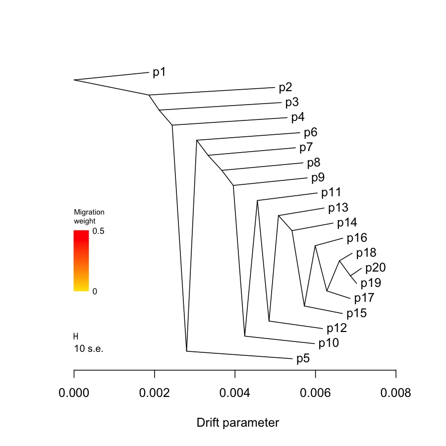
2.1.3. Treemix plots
## system("treemix -i data/treemix.sim1.in.gz -o data/treemix.sim1.out -root p1 ", ignore.stdout = T, ignore.stderr = F)
tm = plot_tree("data/treemix.sim1.out", plus = 0.001, disp = 0.0001)
2.2. long branch
2.2.1. commands
In contrast to short branch, we multiplied all branch lengths by 50. We also simulate 400 independent regions for 20 populations with 20 samples each population without migrations.
ms 400 400 -t 200 -r 200 500000 -I 20 20 20 20 20 20 20 20 20 20 20 20 20 20 20 20 20 20 20 20 20 -en 0.135 20 0.025 -ej 0.1375 20 19 -en 0.2725 19 0.025 -ej 0.275 19 18 -en 0.41 18 0.025 -ej 0.4125 18 17 -en 0.5475 17 0.025 -ej 0.55 17 16 -en 0.685 16 0.025 -ej 0.6875 16 15 -en 0.8225 15 0.025 -ej 0.825 15 14 -en 0.96 14 0.025 -ej 0.9625 14 13 -en 1.0975 13 0.025 -ej 1.1 13 12 -en 1.235 12 0.025 -ej 1.2375 12 11 -en 1.3725 11 0.025 -ej 1.375 11 10 -en 1.51 10 0.025 -ej 1.5125 10 9 -en 1.6475 9 0.025 -ej 1.65 9 8 -en 1.785 8 0.025 -ej 1.7875 8 7 -en 1.9225 7 0.025 -ej 1.925 7 6 -en 2.06 6 0.025 -ej 2.0625 6 5 -en 2.1975 5 0.025 -ej 2.2 5 4 -en 2.335 4 0.025 -ej 2.3375 4 3 -en 2.4725 3 0.025 -ej 2.475 3 2 -en 2.61 2 0.025 -ej 2.6125 2 1 | gzip -c >data/ms.sim2.out.gz
2.2.2. results
find the partitions combination with maximum mean of off-diagnal sub matrix.
file2 = "data/ms.sim2.out.gz"
X2 = parseMsOut(file2)
saveAsTreemixInput(X2, "data/treemix.sim2.in.gz")
println("the results of partitioning by V:")
println(findMaximisingPartitionInV(hatV(X2)))
println("the results of partitioning by Σ:")
println(findMaximisingPartitionInV(hatΣ(X2)))
println("the results of partitioning by W:")
println(findMaximisingPartitionInV(hatW(X2)))
started parsing ms output file
20,6530862
the results of partitioning by V:
[[1], [2, 3, 4, 5, 6, 7, 8, 9, 10, 11, 12, 13, 14, 15, 16, 17, 18, 19, 20]]
the results of partitioning by Σ:
[[1], [2, 3, 4, 5, 6, 7, 8, 9, 10, 11, 12, 13, 14, 15, 16, 17, 18, 19, 20]]
the results of partitioning by W:
[[1, 2, 3, 4, 5, 6, 7, 8], [9, 10, 11, 12, 13, 14, 15, 16, 17, 18, 19, 20]]
the original plot
plotAll(X2, c=:redsblues, colorbar=false)

plots to show the gradients
plotAll2(X2, c=:redsblues, colorbar=false)

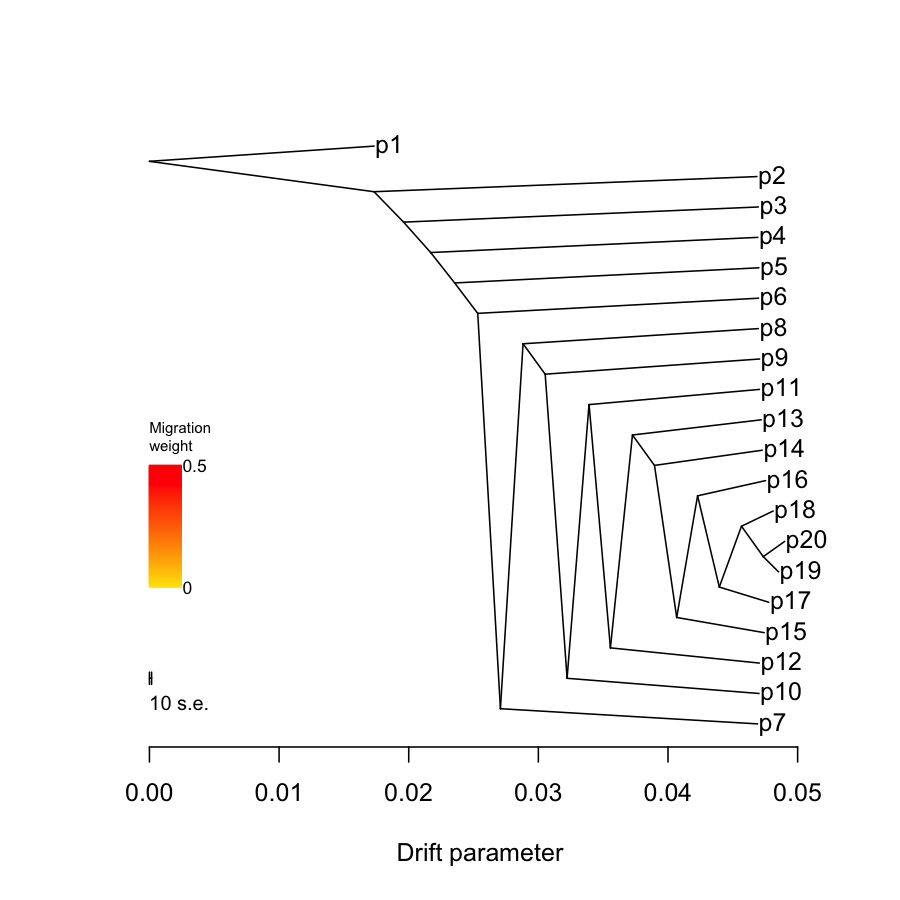
2.2.3. Treemix plots
## par(mfrow=c(1,2))
## system("treemix -i data/treemix.sim2.in.gz -o data/treemix.sim2.root.out -root p1 -k 100", ignore.stdout = T, ignore.stderr = F)
tm = plot_tree("data/treemix.sim2.root.out", plus = 0.002, disp = 0.0001)
## system("treemix -i data/treemix.sim2.in.gz -o data/treemix.sim2.out -k 100", ignore.stdout = T, ignore.stderr = F)
## tm = plot_tree("data/treemix.sim2.out", mbar = F, plus = 0.001, disp = 0.0001)
3. Real Dataset
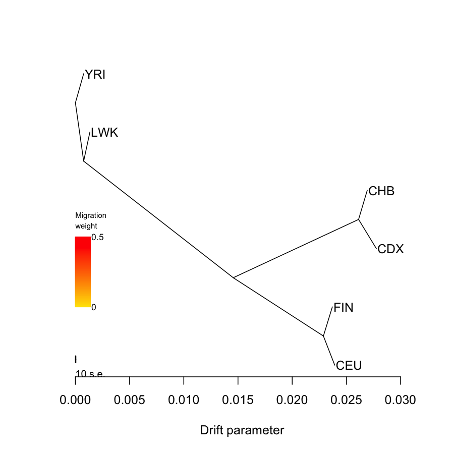
3.1. 1000 Genomes
f = "data/1kg.6pops.in.gz"
Xk = parseTreemixInput(f)
println("the size of input matrix is ", size(Xk))
println("the results of partitioning by V:")
printMaximisingPartitions(hatV(Xk), names(Xk, 1))
println("the results of partitioning by W:")
printMaximisingPartitions(hatW(Xk), names(Xk, 1))

Xk2 = Xk[[1,2,3,5,6], :]
println("\nafter removing LWK from the input")
println("the results of partitioning by V:")
printMaximisingPartitions(hatV(Xk2), names(Xk2, 1))
println("the results of partitioning by W:")
printMaximisingPartitions(hatW(Xk2), names(Xk2, 1))
the populations are:
YRI CHB CDX LWK CEU FIN
the size of input matrix is (6, 4391887)
the results of partitioning by V:
1st partition:["YRI", "LWK"]
2nd partition:["CHB", "CDX", "CEU", "FIN"]
the results of partitioning by W:
1st partition:["YRI", "LWK"]
2nd partition:["CHB", "CDX", "CEU", "FIN"]

after removing LWK from the input
the results of partitioning by V:
1st partition:["YRI"]
2nd partition:["CHB", "CDX", "CEU", "FIN"]
the results of partitioning by W:
1st partition:["YRI", "CEU", "FIN"]
2nd partition:["CHB", "CDX"]
plotAll(Xk, c=:redsblues, colorbar=false)

plotAll2(Xk, c=:redsblues, colorbar=false)

## system("treemix -i data/1kg.6pops.in.gz -o data/treemix.kg.6pops.out -root YRI ", ignore.stdout = T, ignore.stderr = F)
tm = plot_tree("data/treemix.kg.6pops.out", plus = 0.003, disp = 0.0001)
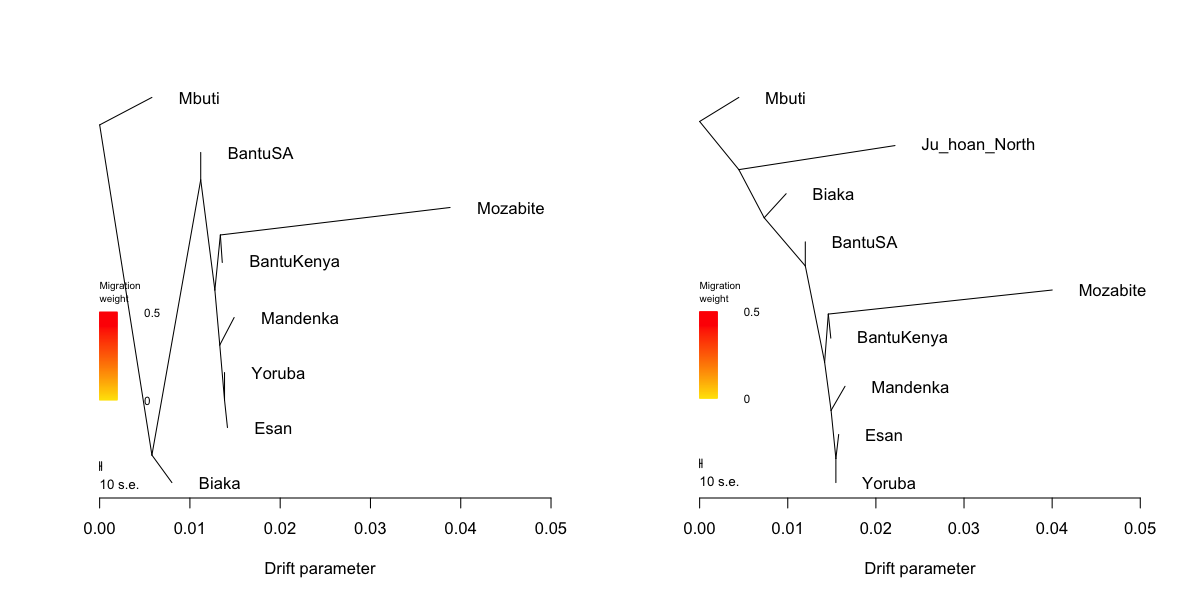
3.2. Human origins
f = "data/treemix.origins.sub1.gz"
Xo = parseTreemixInput(f)
println("the size of input matrix is ", size(Xo))
println("the results of partitioning by V:")
printMaximisingPartitions(hatV(Xo), names(Xo, 1))
println("the results of partitioning by W:")
printMaximisingPartitions(hatW(Xo), names(Xo, 1))
Xo2 = Xo[1:8, :]
println("after removing Mozabite [9] from the input")
println("the results of partitioning by V:")
printMaximisingPartitions(hatV(Xo2), names(Xo2, 1))
println("the results of partitioning by W:")
printMaximisingPartitions(hatW(Xo2), names(Xo2, 1))

Xo2 = Xo[[1,2,3,4,5,6,7,9], :]
println("\nafter removing Ju_hoan_North [8] from the input")
println("the results of partitioning by V:")
printMaximisingPartitions(hatV(Xo2), names(Xo2, 1))
println("the results of partitioning by W:")
printMaximisingPartitions(hatW(Xo2), names(Xo2, 1))

Xo2 = Xo[1:7, :]
println("\nafter removing Ju_hoan_North [8] and Mozabite [9] from the input")
println("the results of partitioning by V:")
printMaximisingPartitions(hatV(Xo2), names(Xo2, 1))
println("the results of partitioning by W:")
printMaximisingPartitions(hatW(Xo2), names(Xo2, 1))
plotAll(Xo, c=:redsblues, colorbar=false)

plotAll2(Xo, c=:redsblues, colorbar=false)

Treemix inference
par(mfrow=c(1,2))
system("treemix -i data/treemix.origins.sub2.gz -o data/treemix.origins.sub2.out -root Mbuti ", ignore.stdout = T, ignore.stderr = F)
tm = plot_tree("data/treemix.origins.sub2.out")
system("treemix -i data/treemix.origins.sub1.gz -o data/treemix.origins.sub1.out -root Mbuti ", ignore.stdout = T, ignore.stderr = F)
tm = plot_tree("data/treemix.origins.sub1.out")